INTRODUCTION

A lot of studies have been done on factors influencing life expectancy considering demographic variables, income composition, and mortality rates. Some of these past research have also been done considering multiple linear regression based on dataset of a year for all the countries. Thus, the motivation behind this study is to examine some of the factors stated to influence life expectancy and also to build a regression model that predicts the life expectancy of an individual while considering data from a period of 2000 to 2015 for all the countries.

Data Set Source

The primary source of the dataset was from the Global Health Observatory (GHO) data repository under World Health Organization (WHO) which keeps track of the health status as well as many other related factors for all countries. The dataset used are made available to public for the purpose of health data analysis and was extracted through Kaggle for this article. The dataset includes information related to life expectancy, health factors for 193 countries. It also includes missing data from less known countries like Vanuatu, Tonga, Togo, Cabo Verde etc. The final merged file(final dataset) consists of 22 Columns and 2938 rows which meant 20 predicting variables. All predicting variables was then divided into several broad categories:​Immunization related factors, Mortality factors, Economical factors and Social factors.

Tools Utilized

• Numpy

• Pandas

• Statsmodels

• Matplotlib

• Seaborn

Process

Using Google Collaboratory, we will build a multiple linear regression model that predicts the life expectancy of an individual using features provided in the dataset. The detailed explanation of the project steps are below.

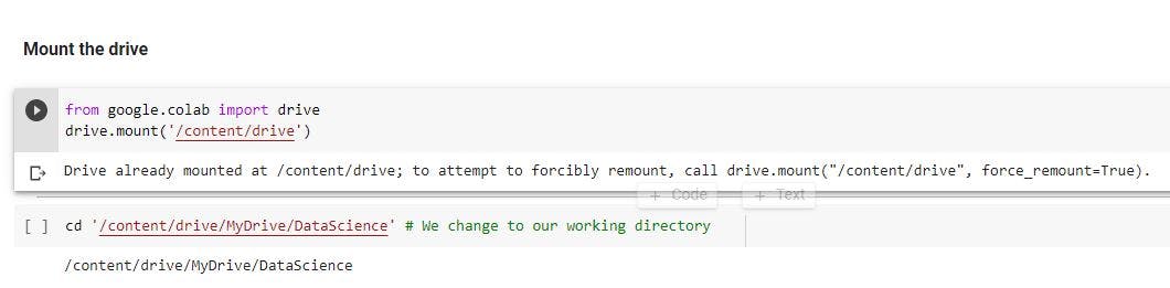
Mount the drive and import relevant libraries

The first step is to create a working directory, say DataScience. In the directory, create LifeExpectancy.ipynb file and mount the Google drive.

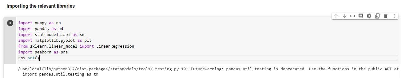
Import the necessary libraries

These are the libraries that would be used for analysis and to build the life expectancy model.

import numpy as np
import pandas as pd
import statsmodels.api as sm
import matplotlib.pyplot as plt
from sklearn.linear_model import LinearRegression
import seaborn as sns
sns.set()

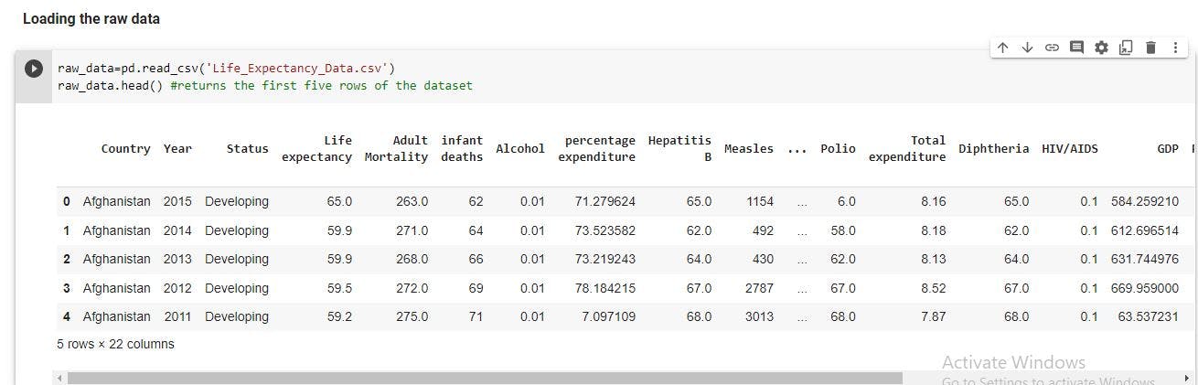
Load the raw data

We should load the dataset with Pandas. This will load the data in form a Pandas dataframe. We can also examine the first five rows of the dataset.

raw_data=pd.read_csv('Life_Expectancy_Data.csv')
raw_data.head() #returns the first five rows of the dataset

Preprocessing

Exploring the descriptive statistics of the variables

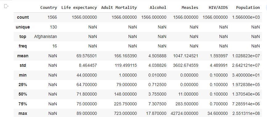
raw_data.describe(include='all') # gives information of all the variables columns in the dataset

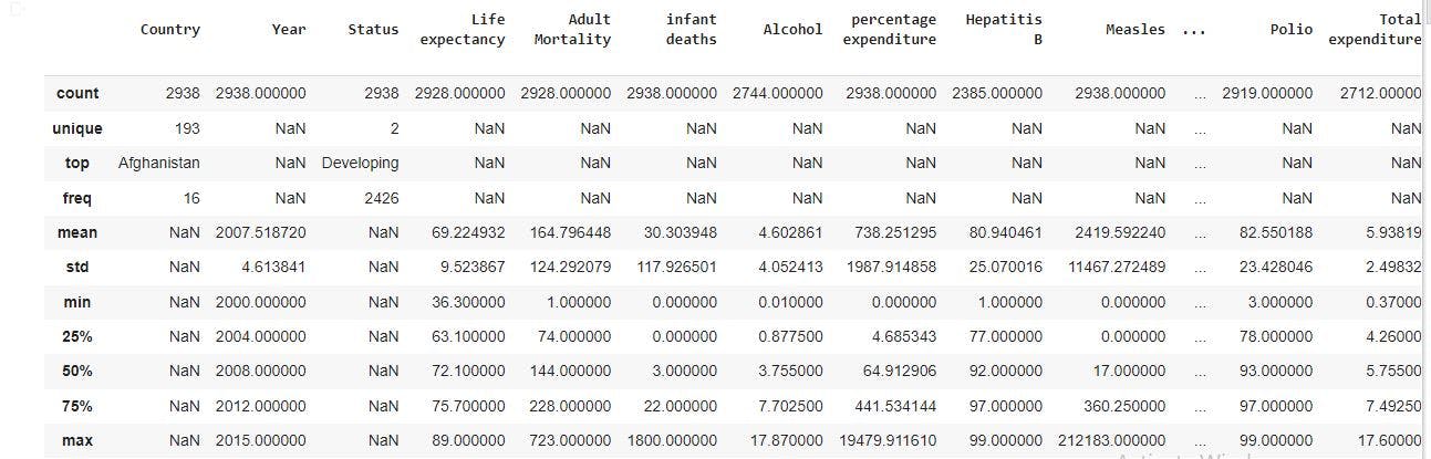
In the image above, there are different count for the variable columns with some having a value of 2938, 2928, 2744, and so on. There are also missing values in some columns represented with NaN. From the statistics, there are 193 unique countries. The top country represented is Afghanistan which has a status of developing country. In addition, for the numeric columns, we have a mean, minimum, maximum value which can be used to further analysis such as checking for outliers.

Dealing with missing values

Let's have the number of missing values in the dataset. We do this by summing the missing values in each column with the code below.

raw_data.isnull().sum()

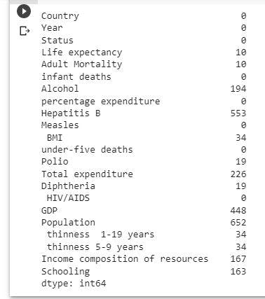
data_no_mv= raw_data.dropna(axis=0)
# Delete the missing values in the columns

After deleting the missing values, we saved the new data in data_no_mv. We should also check the descriptive statistics.

data_no_mv.describe(include='all')

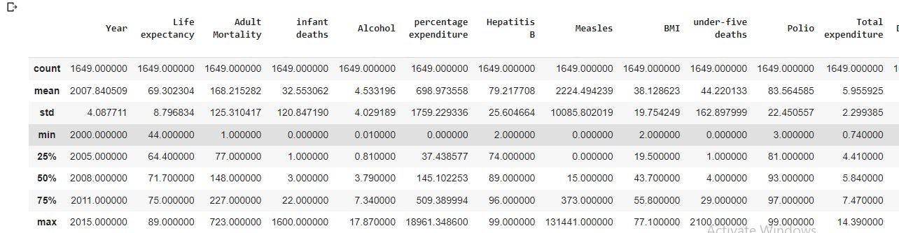
The image above shows a uniform count of 1649 observations for all the columns.

Exploring the probability distribution function

Probability Distribution Function (PDF) is a way check the distribution of data for the variable columns. We will use it check for features that outliers. Let's check the distribution of our target- Life expectancy.

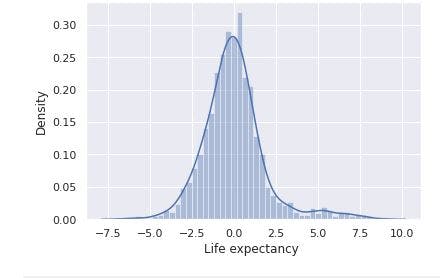
sns.distplot(data_no_mv['Life expectancy '])
# Check the PDF of Life expectancy

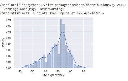
From the image above, Life expectancy has a normal distribution. In addition, from the descriptive statistics we previously have, Life expectancy has a mean of 69 and max of 89. Thus, the target seems not affected by outliers.

We will examine the PDF of other features such as infant deaths, percentage expenditure, Measles, under-five deathsas the descriptive statistics shows a huge gap between the mean value and the max value.

sns.distplot(data_no_mv['infant deaths'])
# Check the PDF of infant deaths

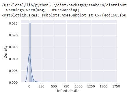
The image above shows infant deaths has a right skewed distribution. This is not unusual considering the feature has a mean of 32 and max of 1600.

sns.distplot(data_no_mv['percentage expenditure'])
# Check the PDF of percentage expenditure

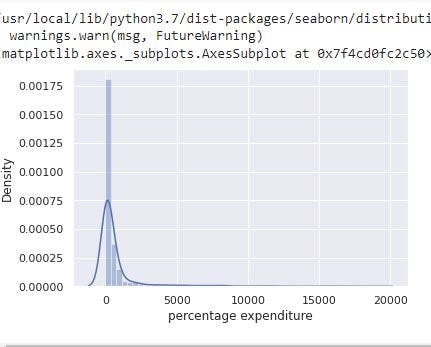
For percentage expenditure, the image shows the feature has a right skewed distribution with a mean of 698.97 and a max of 18961.35.

sns.distplot(data_no_mv['Measles '])
# Check the PDF of Measles

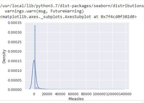
From the image, Measles has a right skewed distribution resulting from the presence of outliers.

sns.distplot(data_no_mv['under-five deaths '])
# Check the PDF of under-five deaths

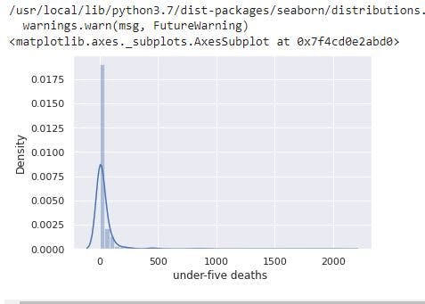
From the image, under-five deaths has a right skewed distribution resulting from the presence of outliers.

sns.distplot(data_no_mv[' HIV/AIDS'])
# Check the PDF of HIV/AIDS

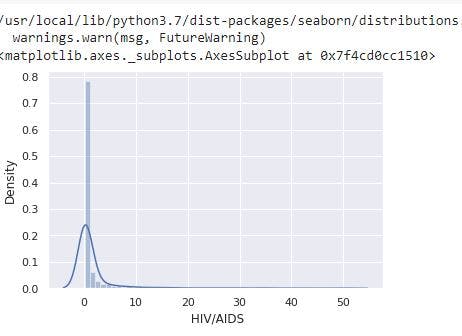
From the image, under-five deaths has a right skewed distribution resulting from the presence of outliers. The descriptive statistics also shows the feature has a mean of 1.98 and a max of 50.60.

Dealing with outliers

Outliers are observations that lie on abnormal distance from other observations in the data. They affect regression as they cause coefficient to be inflated and the model will try to place the line of best fit close to the values. Thus, one way to deal with outliers is to remove the top 1% of observations.

We will use the quantile method to do this. The quantile method allows us to input number between 0 and 1. If we decide to use 0.5, we will get the 50th percentile or 0.4 gives the 40th percentile. We will use the 0.99 as we want to keep observations below the 99th percentile.

q=data_no_mv['infant deaths'].quantile(0.99) # gets the 99th percentile
data_1=data_no_mv[data_no_mv['infant deaths']<q] # keeps observations of infants below the 99th percentile

q=data_1['percentage expenditure'].quantile(0.99)
data_2=data_1[data_1['percentage expenditure']<q]

q=data_2['Measles '].quantile(0.99)
data_3=data_2[data_2['Measles ']<q]

q=data_3['under-five deaths '].quantile(0.99)
data_4=data_3[data_3['under-five deaths ']<q]

q=data_4[' HIV/AIDS'].quantile(0.99)
data_5=data_4[data_4[' HIV/AIDS']<q]
data_5.describe()

We have removed the outliers from the observations to a degree. The next step to reset the index of the observations left in the dataset.

data_cleaned=data_5.reset_index(drop=True)

Checking the ordinary linear square (OLS) assumptions

Multicollinearity

We will check if some of the features that will predict the Life expectancy are correlated. we will do this using Variance Inflation Factor (VIF).

from statsmodels.stats.outliers_influence import variance_inflation_factor    # import VIF 
variables=data_cleaned[['Year', 'Adult Mortality',
       'infant deaths', 'Alcohol', 'percentage expenditure',
       'Hepatitis B', 'Measles ', ' BMI ', 'under-five deaths ', 'Polio',
       'Total expenditure', 'Diphtheria ', ' HIV/AIDS', 'GDP',
       'Population', ' thinness  1-19 years', ' thinness 5-9 years',
       'Income composition of resources', 'Schooling']]  #Selects the numeric columns for which we want to check multicollinearity

vif=pd.DataFrame() #Create a dataframe

vif['VIF']=[variance_inflation_factor(variables.values, i) for i in range (variables.shape[1])] #loops through the variables for VIF 

vif['features']=variables.columns #creates features column and VIF column

print(VIF) #prints the vif dataframe

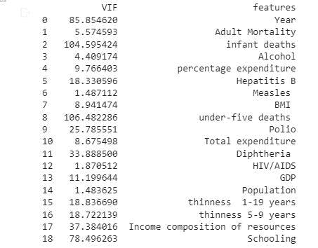
From the image, each feature has a VIF. The VIF shows by how much each feature is correlated to another. According to some sources, features that values between 1 and 5 (1<VIF<5) are okay. Some say features that have a VIF above 6 are unacceptable. Thus, We will drop features with a VIF above 5 from our dataset with our code below.

data_no_multicollinearity=data_cleaned.drop([ 'Year', 'Status',
       'infant deaths', 'percentage expenditure',
       'Hepatitis B',' BMI ', 'under-five deaths ', 'Polio',
       'Total expenditure', 'Diphtheria ', 'GDP',
        ' thinness  1-19 years', ' thinness 5-9 years',
       'Income composition of resources', 'Schooling'], axis=1) #removes the features with VIF above 5 in the dataset

data_no_multicollinearity.describe(include='all')

Create Dummy Variables

We need to add the categorical data - Country for our regression. This will be done by converting the 130 unique countries to dummy variables using pd.get_dummies(df[,drop_first]).

data_with_dummies=pd.get_dummies(data_no_multicollinearity, drop_first=True) #Spots all categorical variables and creates dummies automatically
data_with_dummies.describe(include='all')

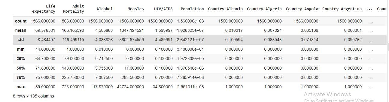
From the image above, we now have a column for each country. It should also be noted that Afghanistan has been removed from the observation. This is because of the drop_first=True we included in the code. This was done to avoid introducing multicollinearity to our regression.

Linear regression model

Declare the inputs and targets

By now, we all know the targets is Life expectancy and the inputs refers the features. So let's separate them.

targets=data_with_dummies['Life expectancy ']
inputs= data_with_dummies.drop(['Life expectancy '],axis=1)

Scale the data

We will standardize the inputs in the dataset before creating a regression model.

from sklearn.preprocessing import StandardScaler
scaler=StandardScaler()
scaler.fit(inputs) #gives the mean and standard deviation of the inputs

inputs_scaled=scaler.transform(inputs) #transforms the data into standardized inputs

Train Test Split

We need to split our data into training and testing data. We are doing this because we need to check the accuracy of the regression model we have built. If we decide not to test our model, we could have a problem of overfitting or underfitting. In simple terms, overfitting is when our model is extremely accurate because it is already familiar with the dataset. Underfitting is when our model is not accurate as the line of best fit misses the data points.

We will split our dataset using train_test_split. In the code below, x_train and x_test refers to the input_scaled. The input_scaled will be split using the test_size of 0.2. This in simple terms means 80% for x_train and 20% for x_test. Also, the targets will be split between y_train and y_test using the test_size. It should be noted that when we split observations, the index of the observations are also included in the split.

from sklearn.model_selection import train_test_split
x_train, x_test, y_train, y_test =train_test_split(inputs_scaled, targets, test_size=0.2, random_state=365)

Create the regression

reg=LinearRegression()
reg.fit(x_train, y_train)

Obtain the predicted values using the code below

y_hat=reg.predict(x_train)

A simple way to check the final result is to plot the predicted values(y_hat) against the observed targets we have in our dataset (y_train).

plt.scatter(y_train, y_hat)
plt.xlabel('Targets (y_train)', size=18)
plt.ylabel('Predictions (y_hat)', size=18)
plt.show()

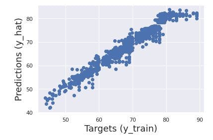
From the image above, we can see the data points are situated around the 45 degree line. Thus, our model has passed the first check.

Residual plot check

One of the regression assumptions (normality and homoscedasticity) is the errors must be normally distributed with a mean of zero. Residuals give an estimate of errors. Thus, we will examine the residual by plotting the differences between the targets and the predictions.

sns.distplot(y_train - y_hat)

The image above shows a normal distribution of errors and a mean of zero. This means our model has another regression assumption.

Checking the variability of the model using R sqaured (R^2)

reg.score(x_train, y_train)

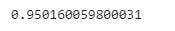
The image shows that our model is explaining 95% of the variability of the data which is is a good result.

Testing our Life expectancy model

After training our model with some data, We will now test the model with the data with split for testing.

y_hat_test= reg.predict(x_test) #predicts the target outcomes

The next step is to plot our predicted target(y_hat_test) with observed targets (y_test) and see whether the data points are along the 45 degree line.

plt.scatter(y_test, y_hat_test)
plt.xlabel('Targets (y_test)', size=18)
plt.ylabel('Predictions (y_hat_test)', size=18)
plt.show()

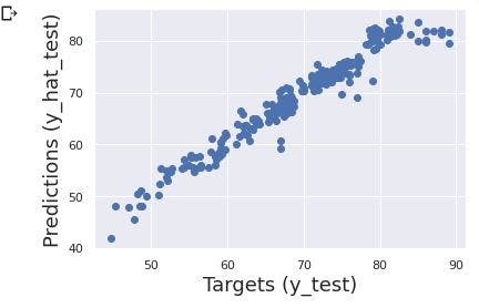
Now, we will create a data frame(df_pf) for our predicted targets using Pandas. This is to have to have description of our output.

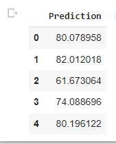
df_pf= pd.DataFrame(y_hat_test, columns=['Prediction']) #creates a Prediction column in the data frame  containing the predicted values.

df_pf.head() #gives the first five rows of the data frame

Let's add the observed targets (y_test) to df_pf data frame and print the first 5 rows.

df_pf['Target']=y_test
df_pf.head()

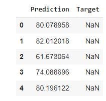
In the image above, we will notice the Target column has NaN values. As stated earlier, when we split observations, the index are also split. Since the split occurred randomly, we would have y_test observations with index different from the index of df_pf. Let's have a look at the y_test with the code below

print(y_test)

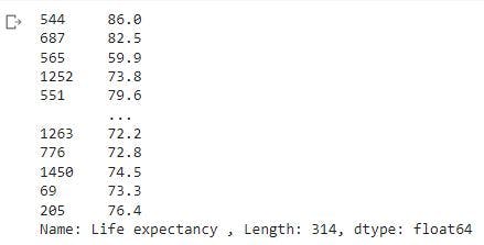
We will reset the index of y_test and print the first 5 rows using the code below

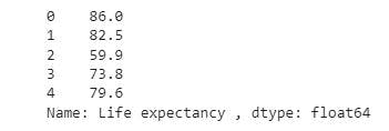
y_test=y_test.reset_index(drop=True)
y_test.head()

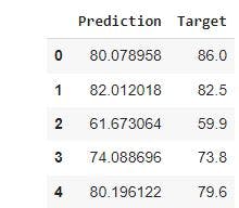
Having reset the index, we will add target to df_pf and print the first 5 rows using the code below

df_pf['Target']=y_test
df_pf.head()

Calculating the residual to estimate error and percentage difference

The next step is to calculate the difference between the observed targets and the predicted targets. After getting the residual, we will include the residual in df_pf.

df_pf['Residual']= df_pf['Target']-df_pf['Prediction']

We will also examine the percentage difference to make it easy to evaluate outputs and the observed targets

df_pf['Difference%']=np.absolute(df_pf['Residual']/df_pf['Target']*100)
print(df_pf)

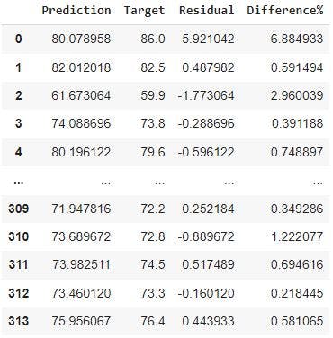
Explore the descriptive statistics of df_pf

We would examine the statistics of the df_pf data frame.

df_pf.describe()

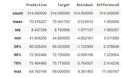
From the image, the minimum and maximum difference in percentage is 0.011583% and 11.545167 respectively. The percentiles (25%, 50%, 75%) for the difference% indicate that for most of our predictions, we were relatively close to the observed targets.

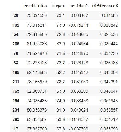
Finally, we will sort df_pf by the percentage difference in the data frame. This will give us insights for the predicted life expectancy age with the least error.

pd.options.display.max_rows=1000 #increases the amount of rows displayed to 1000
df_pf.sort_values(by=['Difference%']) #sorts the data frame with the percentage difference

Conclusion

The life expectancy model built in this project can be helpful for health workers particularly in developing countries or for people living in urban areas. There are several factors influencing life expectancy in the world and this project analyzed the relationship or correlation between the features. The model was also built using multiple linear regression. While building the model, we considered the regression assumptions such as linearity, no endogeneity, no multicollinearity, and no autocorrelation. There are several other approaches that a data scientist can adopt to build a life expectancy model. If you found this project interesting and helpful, leave a like, and check out my other machine learning projects.