Introduction

Convolutional Neural Network (CNN) is a deep learning technique used for image recognition and processing. Over the years, CNN has found a good grip over classifying images for computer visions and now it is being used in urban planning too e.g. through Handwritten Text Recognition (HTR). HTR refers to the ability of a computer to receive and interpret handwritten input from different sources like images, papers, and touch screens. HTR can be applied in improving transportation security in urban areas through number plate recognition. Thus, the aim of this project is to classify images with number texts - MNIST datasets provided by torchvision.

Prerequisites

We will use a deep learning library - Pytorch for in the project and the steps followed will be explained. In addition, some of the hyperparameters we will use would be explained such as the convolutional layers, activation function, and loss functions.

Let's get started by importing relevant libraries

For our project, we will use Google Collaboratory (Colab) because it provides free GPU. To do this, create a Python file in Colab, click on runtime, select change runtime type and then pick GPU. After that, we will import the following libraries to create the model. A brief explanation is given for the libraries we would be using

# Import Pytorch
import torch

# Import torchvision so we can load and transform our dataset
import torchvision
import torchvision.transforms as transforms

# Import optimization library and nn for building our convolution layers
import torch.optim as optim
import torch.nn as nn

# After setting runtime to GPU, set device to use cuda using the code below
if torch.cuda.is_available():
  device = 'cuda' 
else:
  device = 'cpu'

Transforming our image data

Transformers are required to scale image data (pixels) into a format for input in our model. We will transform the images into a tensor and then normalize the pixel values between -1 and 1.

# Transform to Torch tensors and normalize our values between -1 and +1
transform = transforms.Compose([transforms.ToTensor(), transforms.Normalize((0.5,), (0.5,)) ])

Load MNIST dataset using torchvision

We will load training and testing MNIST dataset using torchvision and also include transform to use when loading. We have 60,000 training images and 10,000 testing images, both with a shape of 28 x 28 and no dimension - (greyscale image)

# Load training data 
trainset = torchvision.datasets.MNIST('mnist', train = True, download = True, transform = transform)

# Load testing data 
testset = torchvision.datasets.MNIST('mnist', train = False, download = True, transform = transform)

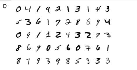
Plot the data with Matplotlib

We will plot examples of the training images using Matplotlib.

figure = plt.figure()
display_images=51
for num in range(1, display_images):
    plt.subplot(5, 10, num)
    plt.axis('off')
    plt.imshow(trainset.data[num], cmap='gray_r')

Creating a data loader

We will create a data loader that specifies batch size during training and testing of data. We will use a batch size of 128 and also select the images randomly. num_workers specifies the number of CPU cores we intend to use to 0

# Prepare train and test loader
trainloader = torch.utils.data.DataLoader(trainset, batch_size = 128, shuffle = True, num_workers = 0)
testloader = torch.utils.data.DataLoader(testset, batch_size = 128, shuffle = False, num_workers = 0)

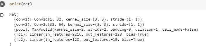
Building the model

We will use the nn.Sequential method to construct our model. The first step is to create our convolutional layers and then define the activation function we will use in the forward propagation sequence.

import torch.nn as nn
import torch.nn.functional as F 

# Create the model with Net
class Net(nn.Module):
    def __init__(self):
        # super is a subclass of the nn.Module and inherits all its methods
        super(Net, self).__init__()

        # Our first CNN Layer using 32 filters of 3x3 size, with the default stride of 1 & padding of 0
        self.conv1 = nn.Conv2d(1, 32, 3)

        # Our second CNN Layer using 64 filters of 3x3 size
        self.conv2 = nn.Conv2d(32, 64, 3)

        # Our Max Pool Layer 2 x 2 kernel of stride 2
        self.pool = nn.MaxPool2d(2, 2)

        # Our first Fully Connected Layer (called Linear), takes the output of our Max Pool, flatten it and     
        connects it to a set of 128 nodes
        self.fc1 = nn.Linear(64 * 12 * 12, 128)

        # Our second FCL, connects the 128 nodes to 10 output nodes
        self.fc2 = nn.Linear(128, 10)

        # Forward propagation      
    def forward(self, x):
        x = F.relu(self.conv1(x))
        x = self.pool(F.relu(self.conv2(x)))
        x = x.view(-1, 64 * 12 * 12)
        x = F.relu(self.fc1(x))
        x = self.fc2(x)
        return x

# Create an instance of the model and move it (memory and operations) to the CUDA device
net = Net()
net.to(device)

Print the model we created

We will print the model to have a look at the convolutional layers

Defining a Loss Function and Optimizer

We will use Cross Entropy Loss as it is a multi-class problem. This gives us the probabilities of the different classes. We will also use an optimizer - Stochastic Gradient Descent (SGD) and specify a stepwise - learn rate (LR) of 0.001 and momentum 0.9.

import torch.optim as optim
criterion = nn.CrossEntropyLoss()
optimizer = optim.SGD(net.parameters(), lr=0.001, momentum=0.9)

Training and testing the model

The dataset we have would be used to train and test the accuracy of our model

# We loop over the training dataset with an epoch size of 10)
epochs = 10

# Create empty arrays to store information as we loop
epoch_log = []
loss_log = []
accuracy_log = []

# Iterate with the specified number of epochs
for epoch in range(epochs):  
    print(f'Starting Epoch: {epoch+1}. ..')

    # We keep adding or accumulating our loss after each mini-batch in running_loss
    running_loss = 0.0

    # We iterate through our trainloader iterator
    # Each cycle is a minibatch
    for i, data in enumerate(trainloader, 0):
        # get the inputs; data is a list of [inputs, labels]
        inputs, labels = data

        # Move our data to GPU
        inputs = inputs.to(device)
        labels = labels.to(device)

        # Clear the gradients before training by setting to zero
        # Required for a fresh start
        optimizer.zero_grad()

        # Forward -> backprop + optimize
        outputs = net(inputs) # Forward Propagation 
        loss = criterion(outputs, labels) # Get Loss (quantify the difference between the results and 
        predictions)
        loss.backward() # Back propagate to obtain the new gradients for all nodes
        optimizer.step() # Update the gradients/weights

        # Print Training statistics - Epoch/Iterations/Loss/Accuracy
        running_loss += loss.item()
        if i % 50 == 49:    # show our loss every 50 mini-batches
            correct = 0 # Initialize our variable to hold the count for the correct predictions
            total = 0 # Initialize our variable to hold the count of the number of labels iterated
            with torch.no_grad():
                # Iterate through the testloader iterator
                for data in testloader:
                    images, labels = data
                    # Move our data to GPU
                    images = images.to(device)
                    labels = labels.to(device)

                    # Foward propagate our test data batch through our model
                    outputs = net(images)

                     # Get predictions from the maximum value of the predicted output tensor
                     # We set dim = 1 as it specifies the number of dimensions to reduce
                    _, predicted = torch.max(outputs.data, dim = 1)
                    # Keep adding the label size or length to the total variable
                    total += labels.size(0)
                    # Keep a running total of the number of predictions predicted correctly
                    correct += (predicted == labels).sum().item()

                accuracy = 100 * correct / total
                epoch_num = epoch + 1
                actual_loss = running_loss / 50
                print(f'Epoch: {epoch_num}, Mini-Batches Completed: {(i+1)}, Loss: {actual_loss:.3f}, Test Accuracy = {accuracy:.3f}%')
                running_loss = 0.0

    # Store training stats after each epoch
    epoch_log.append(epoch_num)
    loss_log.append(actual_loss)
    accuracy_log.append(accuracy)

print('Finished Training')

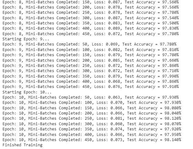
In the image below, we have the loss and accuracy of the model after a 50 minibatch are completed in an epoch. At the completion of the epochs, we have an accuracy of 98.14%. This accuracy of model classifying handwritten digits is very good and we do not have to adjust any of the hyperparameters.

Saving the model

We will save our model so we could use the trained weights in another file for handwritten digit classification.

PATH = './mnist_cnn_net.pth'
torch.save(net.state_dict(), PATH)

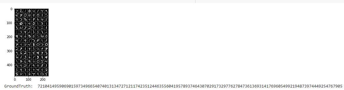
Load some of our test images using Pytorch and view their ground truth labels

# Loading one mini-batch
dataiter = iter(testloader)
images, labels = dataiter.next()
imshow(torchvision.utils.make_grid(images))
print('GroundTruth: ',''.join('%1s' % labels[j].numpy() for j in range(128)))

Reloading the model for reuse

We will reload the model and use it to get predictions

# Create an instance of the model and move it (memory and operations) to the CUDA device.
net = Net()
net.to(device)

# Load weights from the specified path
net.load_state_dict(torch.load(PATH))

Getting the predictions of the test data

test_iter = iter(testloader)

# We use next to get the first batch of data from our iterator
images, labels = test_iter.next()

# Move our data to GPU
images = images.to(device)
labels = labels.to(device)

outputs = net(images)

# Get the class predictions using torch.max
_, predicted = torch.max(outputs, 1)

# Print our 128 predictions
print('Predicted: ', ''.join('%1s' % predicted[j].cpu().numpy() for j in range(128)))

Analyzing our test results with the logs

We have an array of epooc_log, loss_log and accuracy_log we previously created to store information while we loop. We would use these information stored in the array to plot our results.

# To create a plot with secondary y-axis we need to create a subplot
fig, ax1 = plt.subplots()

# Set title and x-axis label rotation
plt.title("Accuracy & Loss vs Epoch")
plt.xticks(rotation=45)

# We use twinx to create a plot a secondary y axis
ax2 = ax1.twinx()

# Create plot for loss_log and accuracy_log
ax1.plot(epoch_log, loss_log, 'g-')
ax2.plot(epoch_log, accuracy_log, 'b-')

# Set labels
ax1.set_xlabel('Epochs')
ax1.set_ylabel('Loss', color='g')
ax2.set_ylabel('Test Accuracy', color='b')

plt.show()

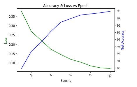
The image below shows the relationship between the loss function and the test accuracy. The test accuracy increases with the number of epochs while the loss function decreases with the number of epochs.

Conclusion

In this blog, we begin by discussing the handwritten digit text recognition and its importance. The tutorial used MNIST dataset downloaded from torchvision to classify and make predictions of handwritten digits from 0 to 9. Using Pytorch, a CNN model was created and was eventually trained on the training dataset. Finally, predictions were made using the trained model.

References

Swati Rajwal (July 12, 2021). Classification of Handwritten Digits Using CNN

Rajeev D. Ratan. Udemy: Modern Computer Vision™ PyTorch, Tensorflow2 Keras & OpenCV4