Introduction

The outbreak of Coronavirus all over the world has resulted in many people expressing the matter on social medias. Twitter, a social media platform, has been used for discussing health, political, and economic issues surrounding the outbreak of the deadly disease. Some of these tweets have expressed displeasure, while some tweets have encouraged people to show resilience. This project aims to build a model that classifies tweets as either positive or negative. This project was done in an attempt to assist health practitioners and government agencies on how best to sensitize the public and also to understand the mindset of people about the disease.

Data Source

The dataset used in this project was got from Kaggle provided by Aman Miglani. The dataset includes tweets from people on Twitter and the names and the usernames of the tweets have been given codes for privacy concerns.

Tools Utilized

• Numpy
• Pandas
• StatsModels
• Matplotlib
• Seaborn
• NLTK

Mount Google drive and change directory

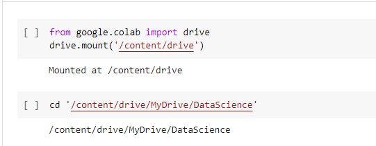
To get started, we will create a working directory, say DataScience, and create a file - NaturalLanguageProcessing.ipynb. The next step is to open the file using Google Collaboratory or Jupyter Notebook. In the file, mount the drive and change directory to DataScience.

from google.colab import drive
drive.mount('/content/drive') # mount the drive
cd '/content/drive/MyDrive/DataScience' # change directory to DataScience

Import relevant libraries

The libraries are the tools we would use for visualization, analysis and for building the model.

import numpy as np
import pandas as pd
import matplotlib.pyplot as plt
import seaborn as sns
import statsmodels.api as sm 
sns.set()

We will also use a tool called stopwords. In order to download it, we have to import nltk

import nltk

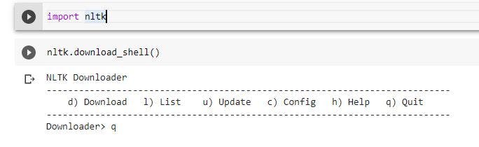
In the image above, when we imported nltk, an HTML input tag was provided. We filled the input with l to check the list of packages. We kept hitting enter till we reached stopwords. The next step was to type d in the input which then asked for the package identifier. We filled the input with stopwords and hit enter to download the package. After downloading the package, we used q to exit the operation.

Load the raw data

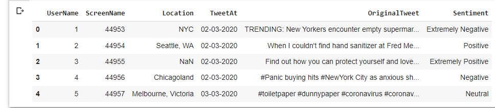
We will read the data with Pandas and then examine the first five rows of the observations.

raw_data= pd.read_csv('Corona_NLP_test.csv')
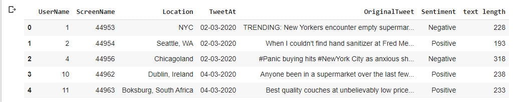
raw_data.head()

Explore the descriptive statistics of the variables

We will examine the statistics of the columns in the dataset to have more understanding about our data.

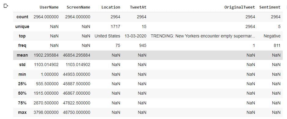
raw_data.describe(include='all')

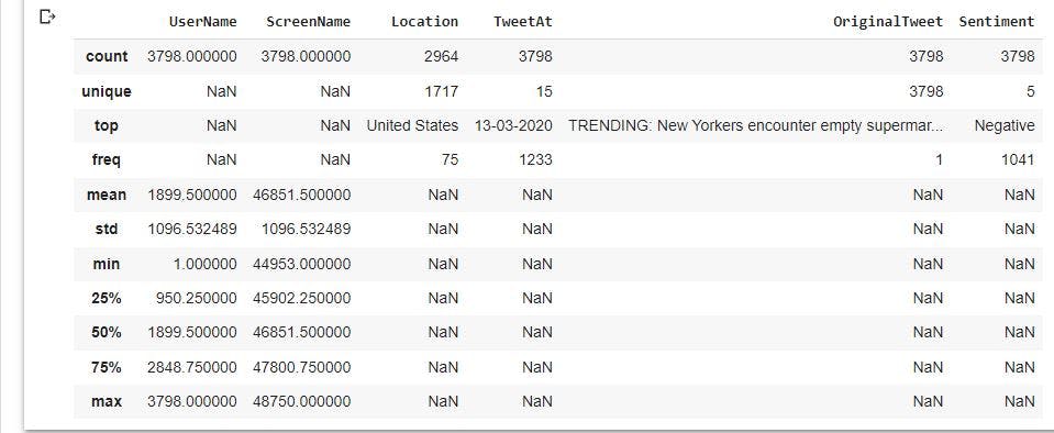
From the image above, we have 3798 observations in the columns with the exception of Location having 2964 values. We also have 5 sentiments which are Negative, Extremely Negative, Neutral, Positive, and Extremely Positive. In addition, most tweets in the dataset were from USA.

Dealing with missing values

To deal with missing values in the dataset, we will get the sum of the missing values and then remove them.

raw_data.isnull().sum()

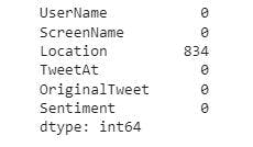
To remove the missing values in Location, we will use the code below:

data_no_mv= raw_data.dropna(axis=0)

After the deletion of observations with missing values, we will have a uniform amount of observation in each column. We will take a look at our data stored in data_no_mv to confirm.

data_no_mv.describe(include='all')

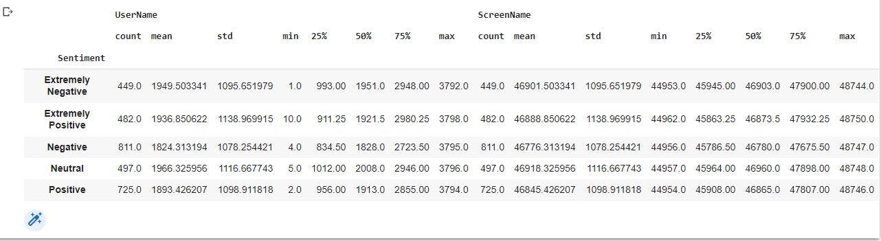
We will also reset the index of the observations in the dataset and store the new data in corona_cleaned. We will also group our data by Sentiments to have a descriptive statistics of the data we are working with.

corona_cleaned=data_no_mv.reset_index(drop=True) # reset the index of the observations
corona_cleaned.groupby('Sentiment').describe() #descriptive statistics of our data by Sentiment

Text Length of the tweets

We will get the length of each tweet from the Original Tweet column and include the values in the dataset.

corona_cleaned['text length']= corona_cleaned['OriginalTweet'].apply(len)

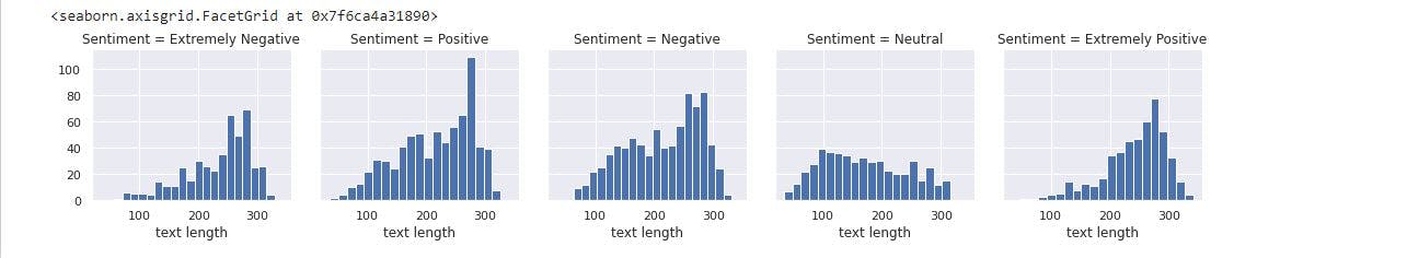
Using FacetGrid from the Seaborn library, we will create a grid of 5 histograms of text based off the sentiments

tweetHist=sns.FacetGrid(corona_cleaned, col='Sentiment')
tweetHist.map(plt.hist, 'text length', bins=20)

The image below shows the distribution of the text length for each sentiment category

We will also create a box plot of text length for each sentiment category.

sns.boxplot(x='Sentiment', y='text length', data=corona_cleaned)

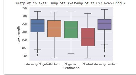
From the image above, it appears Extremely Positive has the highest text length while Neutral has the least text length. In addition, Extremely Negative and Extremely Positive have little outliers.

We will create a countplot of the number of occurrences for the categories of sentiment.

sns.countplot(x='Sentiment', data=corona_cleaned)

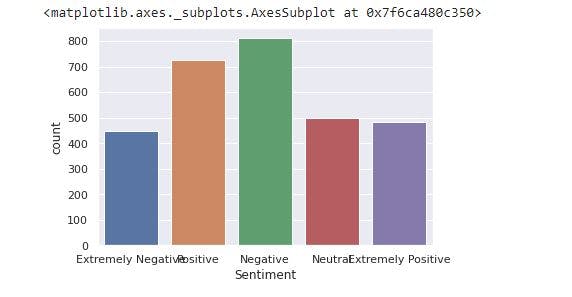
The image shows negative tweets has the highest frequency in the observation and extremely negative tweets have the least frequency.

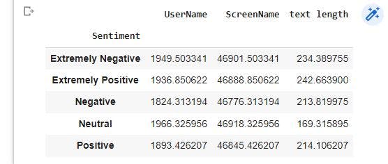
Creating a correlation data frame

In order to create a correlation data frame, we first group by the sentiments to get the mean values of the numerical columns

sentiment=corona_cleaned.groupby('Sentiment').mean()
print (sentiment)

After grouping, we will create a correlation data frame using the code below:

sentiment.corr()

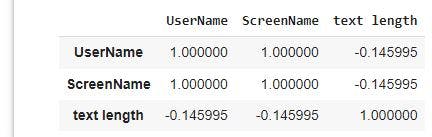
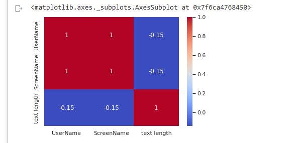
We will create a heatmap off the .corr() dataframe

sns.heatmap(sentiment.corr(), cmap='coolwarm', annot=True)

Merging of sentiments categories

After deleting 834 observations with missing values, we have a small dataset. In order to increase our observations for training and testing our model on tweet classification, we will merge Extremely Negative to Negative and Extremely positive to Positive. We then copy the new data and store in new_sentiment_data.

corona_cleaned['Sentiment'].replace(to_replace={'Extremely Positive':'Positive', 'Extremely Negative':'Negative'}, inplace= True)

new_sentiment_data=corona_cleaned.copy()

Creating a data frame that contains positive and negative sentiment observations

We have tweets in the observations that have neutral sentiments. Thus, we will select observations that have either positive or negative sentiment and then we will reset the index of the new dataset.

new_cleaned_class=new_sentiment_data[(new_sentiment_data['Sentiment']=='Positive')|(new_sentiment_data['Sentiment']=='Negative')] #selects observations with either positive or negative sentiments

sentiment_class=new_cleaned_class.reset_index(drop=True) # reset the index of the dataset

sentiment_class.head() # prints the first five observations

Making use of Python libraries- String and stopwords for tokenization

The OrignialTweet column has some characters "!", "#", "?", "*", "&" and common words such as "any", "both", "each", "other" that do not really differentiate positive tweets from negative tweets. Thus we will import some libraries to remove these characters and words. We import String to remove punctuations from our OriginalTweet column and import stopwords to remove common English words.

import string
from nltk.corpus import stopwords

We will create a function - text_process that loops through each tweet in OrigianalTweet column to remove the characters and common words.

def text_process(tweet):
  nopunc=[char for char in tweet if char not in string.punctuation ]
  nopunc=''.join(nopunc)
  return [word for word in nopunc.split() if word.lower() not in stopwords.words('english')]

We will apply text_process to OriginalTweet using the code below

sentiment_class['OriginalTweet'].apply(text_process)

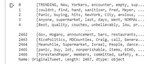
The image above shows a list of tokens for each tweet after punctuations and common words have been removed.

Count vectorization

We will convert each word in the list of tokens into a vector that a machine learning model can understand. We start by importing count vectorizer and then following these three steps:

• Term frequency: count the number of times each word occurs in each message
• Inverse document frequency: weigh the counts
• L2norm: normalize the vectors to unit length.

We will use the code below:

from sklearn.feature_extraction.text import CountVectorizer

bow_transformer=CountVectorizer(analyzer=text_process ).fit(sentiment_class['OriginalTweet'])

After using countvectorizer to fit OriginalTweet, we will transform the tweets using bow_transformer and print the shape of the sparse matrix.

corona_bow=bow_transformer.transform(sentiment_class['OriginalTweet'])
print('Shape of Sparse Matrix: ', corona_bow.shape)

The image above shows the shape of the sparse matrix with 2467 tweets and 12932 vocabulary.

Using term frequency inverse document frequency (Tfidf) for weights and normalization

We will import Tfidf from sklearn, and fit corona_bow to get the weights of our transformed messages.

from sklearn.feature_extraction.text import TfidfTransformer # imports Tfidf from sklearn

tfidf_transformer=TfidfTransformer().fit(corona_bow) # fits corona_bow for the transformation

corona_tfidf=tfidf_transformer.transform(corona_bow) #transforms corona_bow into weights

Creating models using naive_bayes and pipeline

In this project, we will use two methods to create models for our tweets by using sklearn naive_bayes and pipeline. We will adopt these two methods just to give more insights on how the model can be built.

To create the model - tweet_sentiment_model using naive_bayes, we use the following codes below

from sklearn.naive_bayes import MultinomialNB 

tweet_sentiment_model=MultinomialNB().fit(corona_tfidf, sentiment_class['Sentiment'])

tweet_sentiment_model.predict(corona_tfidf)

The image above shows an array of the predicted sentiments by the model for each observation. This concludes the end of the naive_bayes method.

Using Sklearn pipeline to build the model

Before we import pipeline for creating the model, we will split OriginalTweet and Sentiment columns in sentiment_class into training and testing dataset. This is because pipeline does all the preprocessing such as count vectorization, Tfidf transformation itself.

from sklearn.model_selection import train_test_split

tweet_train, tweet_test,label_train, label_test= train_test_split(sentiment_class['OriginalTweet'], sentiment_class['Sentiment'], test_size=0.2, random_state=101)

Importing pipeline and creating the steps argument using the code below

from sklearn.pipeline import Pipeline

pipeline=Pipeline([
    ('bow', CountVectorizer(analyzer=text_process)),
    ('tfidf',TfidfTransformer()),
    ('classifer', MultinomialNB())
])

Fitting and making predictions

pipeline.fit(tweet_train, label_train) # fits with training data

predictions= pipeline.predict(tweet_test) # predicts with testing data

Making a classification report

After making our predictions, we will create a classification report to check the accuracy of our model making predictions.

from sklearn.metrics import classification_report

print(classification_report(label_test, predictions))

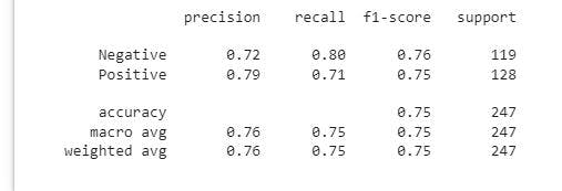
The image above shows our model has an prediction accuracy of 75%. The model is good at making predictions and can be improved on by exploring other classifiers such as random forest classifier.

Conclusion

The application of machine learning in solving problem related to disease outbreak will continue to remain relevant in the world. With models such as the one built in this project, we can predict the sentiments of people on social medias. There a lot more dimensions that we will apply machine learning to like for predicting human mobility patterns during natural disasters. If you found this project interesting, helpful, or have any suggestion on how it can be improved on, kindly click the like button or drop a comment. Thanks!!!