Introduction

Over the years, remote sensing (RS) images have played an important role in a large diversity of applications, and thus, have attracted remarkable research attentions. As a result of this, several datasets have been developed to advance the development of interpretation algorithms for RS images. The classification of RS images can be done either by developing a convolutional neural network (CNN) model from scratch or by utilizing CNN architectures (pretrained models) e.g., ResNet18, VGG16, and MobileNet already trained on ImageNet dataset. These pretrained models can be used to classify satellite images through transfer learning. Thus, in this project, we will fine tune the weights of ResNet50 in order to classify the satellite images.

Description of the satellite image dataset

The satellite image classification dataset-RSI-CB256 has 4131 annotated images with 3 different classes (cloudy, desert, green_area) mixed from Sensors and google map snapshot. There are 1500 cloudy files; 1131 desert files; and 1500 green_area files. The dataset is available for download on Kaggle and was provided for the RS community for data driven research.

Getting Started with the project

The satellite image dataset has no specified train and validation dataset. Thus, we will create separate directories (train and val) with sub-directories that contain images for each class. We will also create a Python file Satellite_imagery.ipynb where we will write our code.

Connect Google drive and import relevant libraries

In Satellite_imagery.ipynb:

Connect and mount Google drive

from google.colab import drive
drive.mount('/content/drive')

Import libraries:

from __future__ import print_function, division
import torch
import torch.nn as nn
import torch.optim as optim
from torch.optim import lr_scheduler
import numpy as np
import torchvision
from torchvision import datasets, models, transforms
import matplotlib.pyplot as plt
import time
import os
import copy
plt.ion()
device = torch.device("cuda:0" if torch.cuda.is_available() else "cpu")

Setup a working directory

In Satellite_imagery.ipynb, we will set our directory to satellite_imagery_project. This is the folder that contains the .ipynb file and the dataset.

cd '/content/drive/MyDrive/satellite_imagery_project/'

Data Preprocessing

In order to feed our images into the model, we need to preprocess our images in train and val. We resize our images into another shape; perform augmentation by randomly flipping them; transform our images into tensors and then normalize them.

data_transforms = {
    'train': transforms.Compose([
        transforms.RandomResizedCrop(224),
        transforms.RandomHorizontalFlip(),
        transforms.ToTensor(),
        transforms.Normalize([0.485, 0.456, 0.406], [0.229, 0.224, 0.225])
    ]),
    'val': transforms.Compose([ 
        transforms.Resize(256), 
        transforms.CenterCrop(224),
        transforms.ToTensor(),
        transforms.Normalize([0.485, 0.456, 0.406], [0.229, 0.224, 0.225])
    ]),
}

Set Data loaders

We will create a dataloader that feeds our images in batches into the model.

# Set to your image path
data_dir = './dataset'

# Use ImageFolder to point to our full dataset 
image_datasets = {x: datasets.ImageFolder(os.path.join(data_dir, x), data_transforms[x]) for x in ['train', 'val']}

# Create our dataloaders
dataloaders = {x: torch.utils.data.DataLoader(image_datasets[x], batch_size=4, shuffle=True, num_workers=4) for x in ['train', 'val']}

# Get our dataset sizes
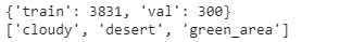
dataset_sizes = {x: len(image_datasets[x]) for x in ['train', 'val']}
print(dataset_sizes)

class_names = image_datasets['train'].classes
print(class_names)

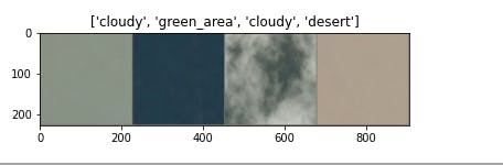
Visualize some images

We will visualize some images with their labels in train using the code below

def imshow(inp, title=None):
    """Imshow for Tensor."""
    inp = inp.numpy().transpose((1, 2, 0))
    mean = np.array([0.485, 0.456, 0.406])
    std = np.array([0.229, 0.224, 0.225])
    inp = std * inp + mean
    inp = np.clip(inp, 0, 1)
    plt.imshow(inp)
    if title is not None:
        plt.title(title)
    plt.pause(0.001)  # pause a bit so that plots are updated

# Get a batch of training data
inputs, classes = next(iter(dataloaders['train']))

# Make a grid from batch
out = torchvision.utils.make_grid(inputs)

imshow(out, title=[class_names[x] for x in classes])

Create function to train our model

We will create a function that saves the weight of the model with the best accuracy.

def train_model(model, criterion, optimizer, scheduler, num_epochs=25):
    since = time.time()

    best_model_wts = copy.deepcopy(model.state_dict())
    best_acc = 0.0

    for epoch in range(num_epochs):
        print('Epoch {}/{}'.format(epoch, num_epochs - 1))
        print('-' * 10)

        # Each epoch has a training and validation phase
        for phase in ['train', 'val']:
            if phase == 'train':
                model.train()  # Set model to training mode
            else:
                model.eval()   # Set model to evaluate mode

            running_loss = 0.0
            running_corrects = 0

            # Iterate over data.
            for inputs, labels in dataloaders[phase]:
                inputs = inputs.to(device)
                labels = labels.to(device)

                # zero the parameter gradients
                optimizer.zero_grad()

                # forward
                # track history if only in train
                with torch.set_grad_enabled(phase == 'train'):
                    outputs = model(inputs)
                    _, preds = torch.max(outputs, 1)
                    loss = criterion(outputs, labels)

                    # backward + optimize only if in training phase
                    if phase == 'train':
                        loss.backward()
                        optimizer.step()

                # statistics
                running_loss += loss.item() * inputs.size(0)
                running_corrects += torch.sum(preds == labels.data)

            if phase == 'train':
                scheduler.step()

            epoch_loss = running_loss / dataset_sizes[phase]
            epoch_acc = running_corrects.double() / dataset_sizes[phase]

            print('{} Loss: {:.4f} Acc: {:.4f}'.format(phase, epoch_loss, epoch_acc))

            # deep copy the model
            if phase == 'val' and epoch_acc > best_acc:
                best_acc = epoch_acc
                best_model_wts = copy.deepcopy(model.state_dict())

        print()

    time_elapsed = time.time() - since
    print('Training complete in {:.0f}m {:.0f}s'.format(time_elapsed // 60, time_elapsed % 60))
    print('Best val Acc: {:4f}'.format(best_acc))

    # load best model weights
    model.load_state_dict(best_model_wts)
    return model

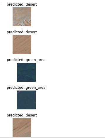
Create function to visualize our model's prediction

We will create a function to plot the images with their predicted labels.

def visualize_predictions(model, num_images=6):
    was_training = model.training
    model.eval()
    images_so_far = 0
    fig = plt.figure()

    with torch.no_grad():
        for i, (inputs, labels) in enumerate(dataloaders['val']):
            inputs = inputs.to(device)
            labels = labels.to(device)

            outputs = model(inputs)
            _, preds = torch.max(outputs, 1)

            for j in range(inputs.size()[0]):
                images_so_far += 1
                ax = plt.subplot(num_images//2, 2, images_so_far)
                ax.axis('off')
                ax.set_title('predicted: {}'.format(class_names[preds[j]]))
                imshow(inputs.cpu().data[j])

                if images_so_far == num_images:
                    model.train(mode=was_training)
                    return
        model.train(mode=was_training)

Fine tuning the convet

We will load Resnet18 without freezing any of the layers and change the fully connected layer to output to class size 3 (number of categories )

model_ft = models.resnet18(pretrained=True)
num_ftrs = model_ft.fc.in_features

# Here the size of each output sample is set to 3.
# Alternatively, it can be generalized to nn.Linear(num_ftrs, len(class_names)).
model_ft.fc = nn.Linear(num_ftrs, 3)

model_ft = model_ft.to(device)

criterion = nn.CrossEntropyLoss()

# Observe that all parameters are being optimized
optimizer_ft = optim.SGD(model_ft.parameters(), lr=0.001, momentum=0.9)

# Decay LR by a factor of 0.1 every 7 epochs
exp_lr_scheduler = lr_scheduler.StepLR(optimizer_ft, step_size=7, gamma=0.1)

Training and Evaluation

Using the function train_model we created earlier, we will set the model and the hyperparameters

model_ft = train_model(model_ft,
                       criterion,
                       optimizer_ft,
                       exp_lr_scheduler,
                       num_epochs=25)

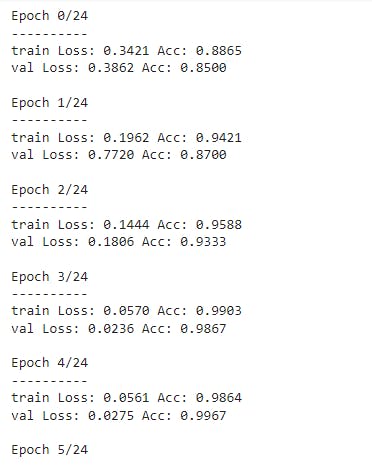
In the image above, the best val accuracy was (99.97%) during the 5th epoch. Thus, the weights the model in the state was saved and returned.

Visualization of the images with predicted labels

The visualization of images with the predicted label would be done by using the function visualize_predictions

visualize_predictions(model_ft)
plt.ioff()
plt.show()

Conclusion

The model, ResNet18 was used as a base layer for the classification of satellite images, and had a validation accuracy of 99.97%. Thus, the weights of the model could be used to classify similar remote sensing images. It should also be noted the model was trained on a satellite image dataset of 4131 images. However, the model could be improved upon by training on a larger satellite image dataset e.g., 10,000 images. Doing this allows the model to learn more low level features in satellite images. On a final note, there is an increasing demand for the automatic classification of remote sensing images, and this has resulted in the development of more interpretation algorithms.

References

Rajeev D. Ratan. Udemy: Modern Computer Vision™ PyTorch, Tensorflow2 Keras & OpenCV4